What Size Do XRD, SEM and TEM Actually Measure?

X-ray diffraction (XRD) records how a crystal scatters X-rays, conventionally with the diffraction angle 2θ on the horizontal axis and diffracted intensity on the vertical axis. A periodic arrangement of atoms produces diffraction peaks, and the width of a peak is related to the distance over which that arrangement remains coherent. The coherent domain size estimated from peak width therefore describes the ordered region that diffracts coherently along a particular crystallographic direction.

That ordered region is not what an electron microscope measures. Conventional secondary-electron images in a scanning electron microscope (SEM) mainly reflect surface topography, while a transmission electron microscope (TEM) forms its image from transmitted and scattered electrons. When a diameter is measured along the particle outline, both techniques return a geometric dimension of the outline; a single TEM image also collapses information through the thickness of the specimen into one planar projection.

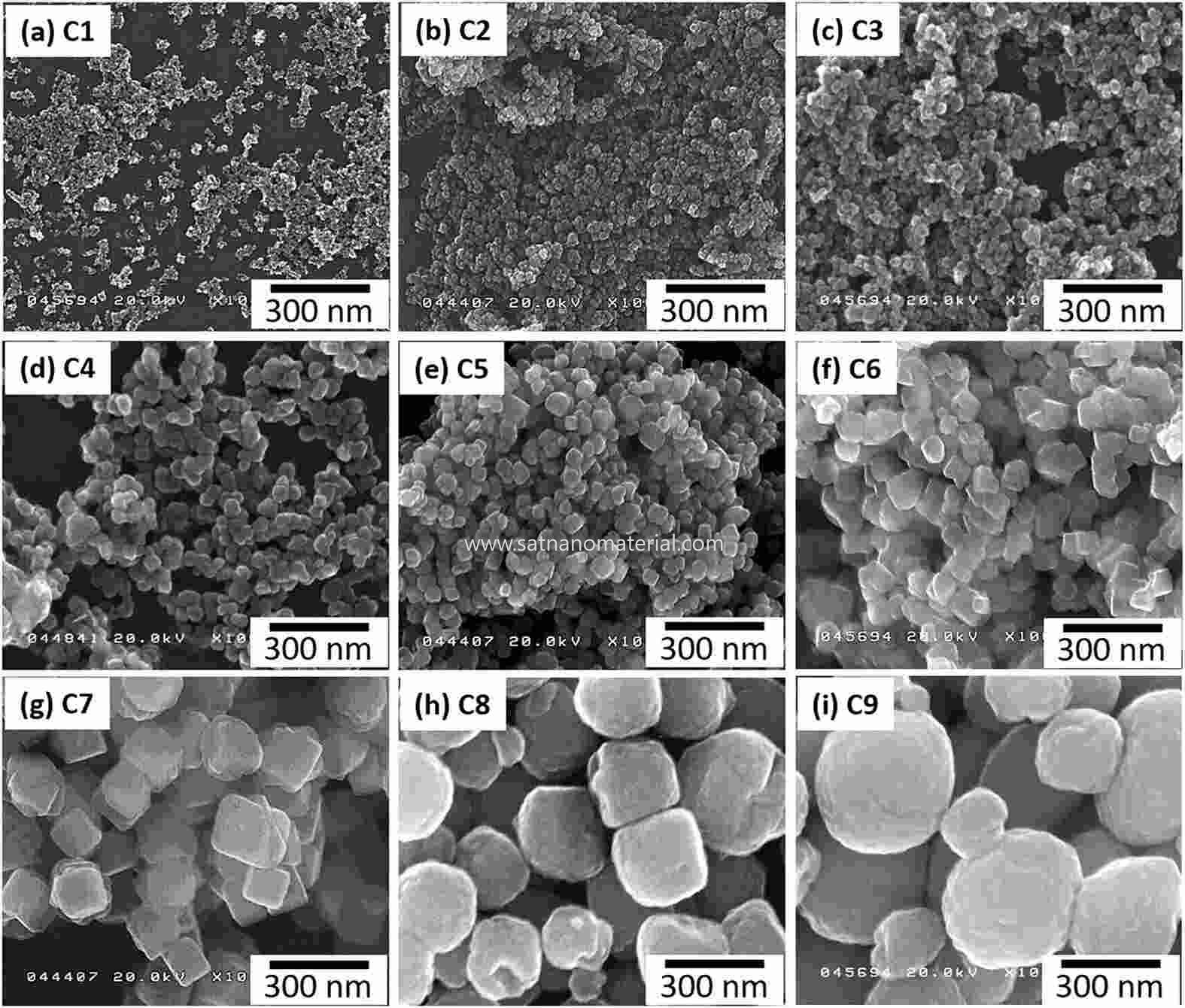
Figure 1.SEM morphology of near-cubic Fe3O4 nanoparticles of different particle sizes.

Such an outline may enclose a single grain, or several grains of different orientation. Particles are defined by their shape, grains by crystallographic orientation and grain boundaries, and coherent domains by the coherence range of the reflection being analysed. Certain defects can even make the coherence length inside a grain shorter than the grain's own geometric size.

The usual way to connect coherence length with peak width is the Scherrer equation, D = Kλ / (βsizecos θ), where λ is the X-ray wavelength, θ is half of the diffraction angle 2θ, and βsizeis the size broadening of the 2θ peak expressed in radians; K is a dimensionless factor that depends on the shape and on how the breadth is defined. Only the size-broadening term enters this relation, and the full width at half maximum and the integral breadth each require their own matching value of K.

Why Is the XRD Size Smaller for the Same Particle?

Several Grains Inside One Particle, and Particle Aggregation

The D in the equation describes the coherent region only, so when a single outline contains many grains, D can be far smaller than the particle diameter. A study of palladium nanodiscs gives a concrete example: the discs produced were about 200 nm across and about 30 nm thick, with an initial mean grain size of roughly 10 ± 2 nm. Both dimensions of the outline are larger than the internal grains, and cycles of hydrogen absorption and desorption further coarsen the grains within the discs.

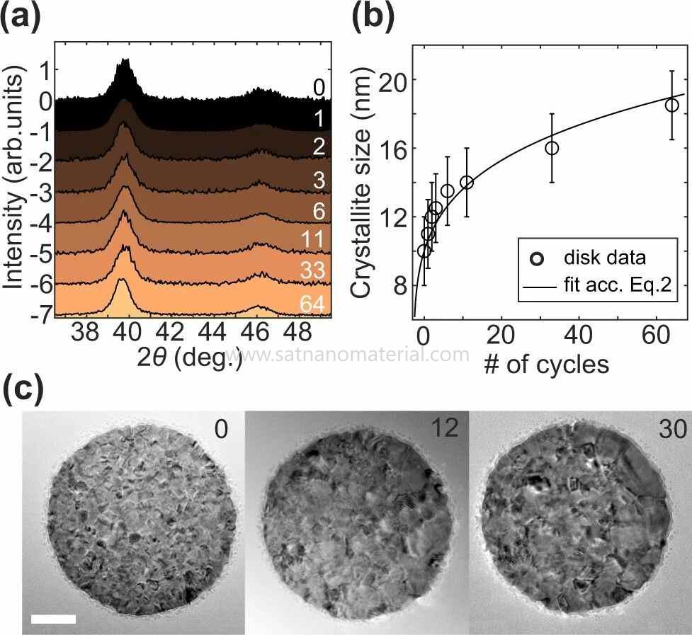
Figure 2.Grazing-incidence XRD, mean domain size and TEM sequences of the same palladium nanodiscs through hydrogen absorption and desorption cycles.

The same gap appears when nanocrystals of different orientation aggregate into a larger body without forming a continuous coherent lattice, so that the entity measured by SEM is larger than any individual domain. For outlines of this kind, high-resolution TEM and local electron diffraction supply the missing information on internal orientation and interfaces; ordinary SEM morphology cannot resolve grain boundaries buried inside the outline.

An Amorphous Shell Around a Crystalline Core

Even an isolated particle with a single crystalline core can still present an outline enlarged by an amorphous outer layer. An amorphous shell lacks long-range periodicity and contributes mainly diffuse scattering, while the periodic arrangement of the core produces the Bragg peaks of the corresponding phase. The diameter of the whole particle includes the shell, whereas the coherence length estimated from the core reflections describes the crystalline region alone.

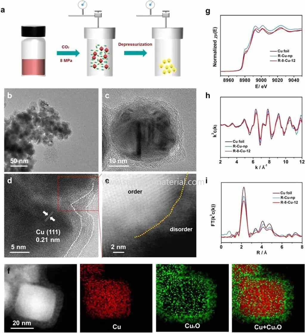
Figure 3.Preparation of copper-based particles, the crystalline-core/amorphous-shell structure with its valence distribution, and the copper K-edge absorption spectrum after reduction.

Copper-based core–shell particles show exactly this difference in scale. After copper nanoparticles were treated in 8 MPa of carbon dioxide for 12 h, their overall size was still about 40 nm, while the outer layer had become an amorphous CuxO shell roughly 4 nm thick. That shell is the amorphous copper oxide component present before electroreduction, and crystalline metallic copper remains inside; measuring the full outline includes the shell, whereas the metallic copper reflections come mainly from the crystalline core.

Broadening Other Than Size Also Lowers the Calculated Value

The diffraction peaks of the crystalline core are also broadened by microstrain: interplanar spacings differ slightly from place to place, and the angles that satisfy the diffraction condition are dispersed accordingly. Treat that width as size broadening, and the β entered into the equation is too large, which makes D too small. In a worked example with K, λ and θ held fixed, a β overestimated by 20% gives a D about 17% too small, because 1 / 1.2 is approximately 0.83.

Instrumental broadening is a further contribution, and its angular dependence can be established with a standard measured under the same optical configuration. Instrument and specimen profiles combine by convolution, and there is no universal way to subtract one full width at half maximum from another. Once the instrumental response has been corrected, the angular dependence of several reflections supports analyses such as the Williamson–Hall method, which estimates the size and microstrain contributions separately.

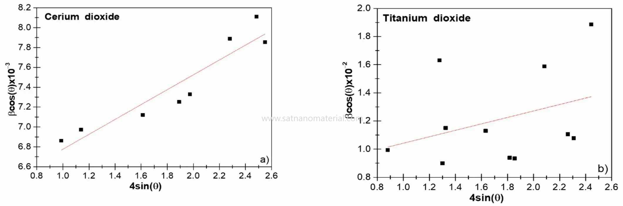
The simplified Williamson–Hall analysis used to separate size from microstrain usually assumes that size and microstrain are roughly the same in every direction, and the peak-shape model employed must also match the data.

In a comparative study of CeO2 and TiO2 nanoparticles, the multi-peak data for TiO2departed from the simplified linear relation; dislocations, stacking faults or direction-dependent size all alter individual reflections. Even where the directional model is appropriate, a measured peak that already sits close to the instrumental line width leaves very little residual size broadening, so a small difference in the fit produces a large change in D.

What Do Direction and Statistics Contribute?

Length Along the Plane Normal vs Projected Particle Size

Even with the instrumental response corrected, the length of a crystal can still differ from one direction to another. A single reflection gives a D corresponding to the coherence length along that plane normal, whereas an electron micrograph may yield the longest projected diameter or an equivalent diameter. For rod-shaped and plate-shaped particles the length, width and thickness differ substantially, so numbers taken from different directions can differ by a factor of several.

Layered double hydroxide (LDH) sheets possess a lateral dimension and a thickness at the same time. One study measured sheet shape and height by AFM, estimated the in-plane domain size from the (110) reflection in XRD, and compared how both changed with the shear rate used in synthesis. The in-plane coherence length here is related to the lateral morphology of the sheet and cannot simply be relabelled as the sheet thickness.

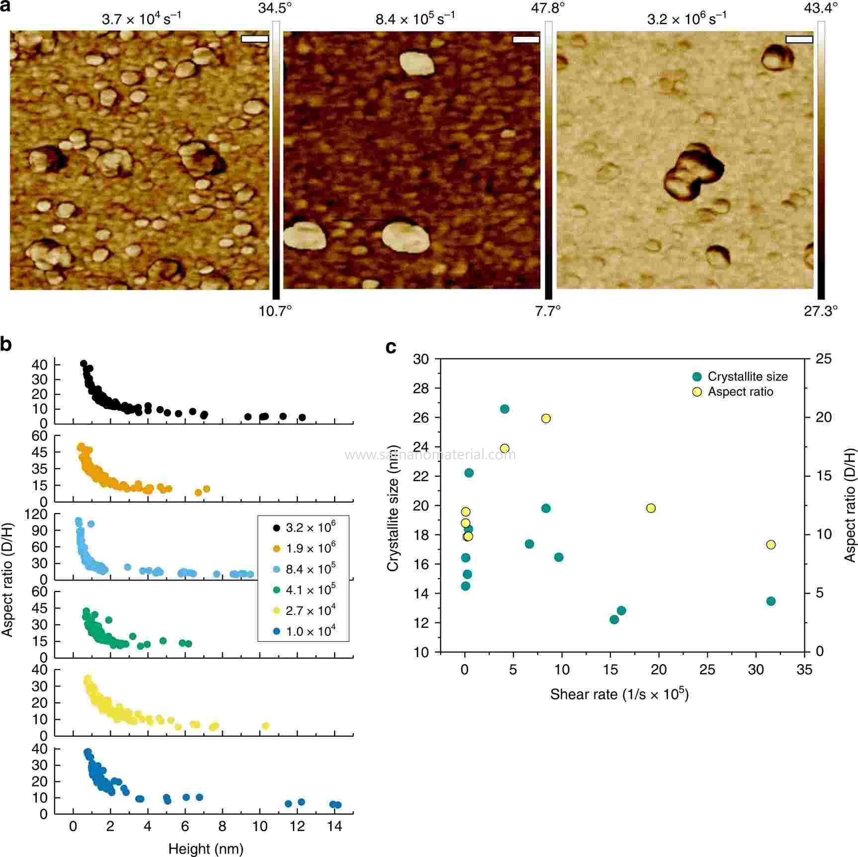
Figure 5.AFM morphology, aspect ratio and in-plane domain size of LDH sheets synthesized at different shear rates.

For a layered crystal whose basal plane lies close to perpendicular to the c axis, the (00l) reflections along c mainly reflect the coherence length in the stacking direction. When thin sheets lie flat, however, the TEM projection tends to emphasise the much larger lateral outline; comparing that lateral dimension with the stacking-direction length can produce widely divergent numbers even when the sheet is well crystallized throughout. Only when the layer remains continuously ordered up to the outline in that direction does the coherence length approach the particle size in the same direction.

Number Distribution vs the Weighted Statistics of the Diffraction Profile

Along a single direction, measuring particle after particle on TEM images and taking the arithmetic mean gives an average weighted by number. XRD obtains its size information from diffracted intensity and a peak-profile model instead, so the result shifts with the definition of breadth, the shape assumed and the distribution assumed. The same CeO2 and TiO2 study compared model domain-size distributions with TEM particle-size distributions, and the two are not the same kind of number histogram.

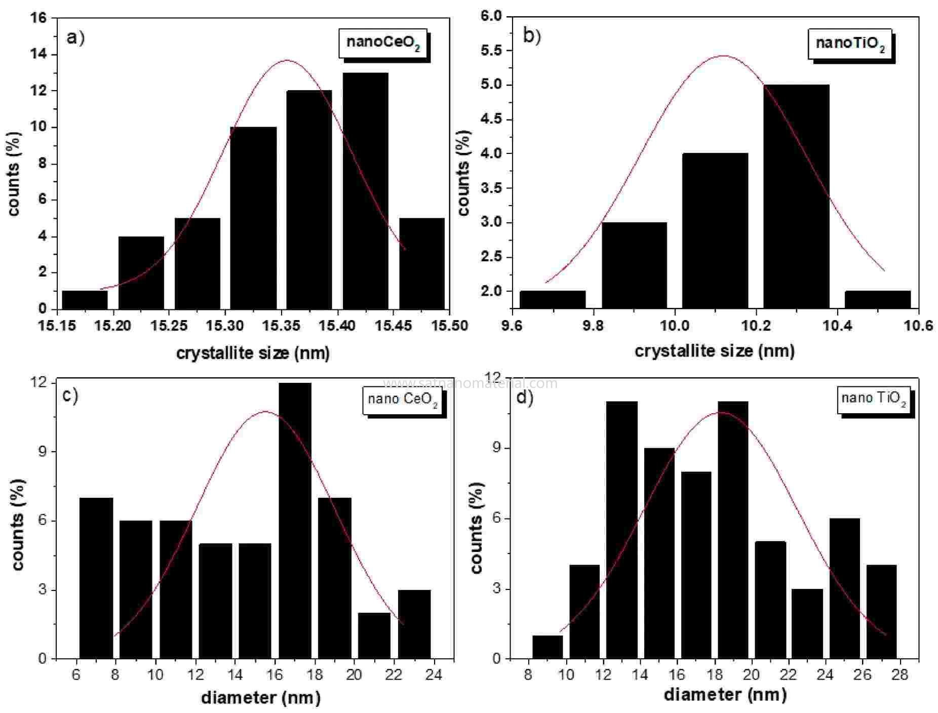
Figure 6.Model domain-size distributions of CeO2 and TiO2, together with TEM particle-size distributions.

In a sample with a broad size distribution, a small number of large crystals can supply the narrow component of the profile while the small crystals supply the broad component; and if the microscope field of view favours small, easily dispersed particles with clear outlines, the resulting mean is biased low again. The XRD size can therefore also exceed the electron-microscopy mean, and the ranking of the two sizes changes with sample composition, sampling and the profile model chosen.

The two measurements describe closer to the same region, and the same statistic, only when the sampling is representative, the particles are close to equiaxed single crystals and the distribution is narrow. In one study of near-cubic Fe3O4nanoparticles spanning roughly 10–65 nm, XRD domain sizes were close to TEM particle sizes, and high-resolution TEM recorded a consistent lattice-fringe orientation within each particle.